Curate the Learning Signal for Reinforcement Learning
Variance Minimization, Adaptive Sampling, and Self-Hinting
TLDR. View RAFT as an EM-like rejection-sampling loop over latent reasoning traces: with a static per-prompt inference budget, gradient estimates become highly heteroskedastic across prompts (some are stable, others are noisy or degenerate). GVM-RAFT makes this bottleneck explicit and proposes prompt-specific dynamic sample allocation to minimize stochastic gradient variance under a fixed compute budget [1]. From the same gradient-first lens, we can also describe “which prompts we care about” via a non-linear pass-rate objective $J_f=\mathbb E_x[f(p_\theta(x))]$, whose derivative induces a prompt weight $w(p)=f’(p)$; Reinforce-Ada operationalizes this with weighting, adaptive sampling, and downsample-correct to obtain stable, non-degenerate updates [2]. Finally, SAGE reframes standardized GRPO as a gated update process and uses (self-)hinting (changing the condition from $x$ to $(x,h)$) to increase the gate-opening probability by steering $p_\theta(x,h)$ toward $1/2$ [3].
This note ties three ideas into one story:
- GVM-RAFT [1]: start from RAFT as rejection sampling / EM-style latent-variable optimization, then derive a variance-minimizing dynamic sampling rule under a compute budget
- Reinforce-Ada [2]: choose a non-linear objective $J_f$ and realize it via weighting and/or adaptive sampling, using downsampling to improve signal-to-noise and stabilize updates
- SAGE / self-hinting [3]: treat standardized GRPO as a gated update process and use hints to open the gate more often
There are two threads running through the note. The gate thread is the most intuitive: a prompt only produces useful learning signal when the sampled group contains reward variation, otherwise the advantage collapses to zero. The variance thread is the deeper estimator-side story: once the gate is open, the remaining question is how to allocate samples, choose baselines, balance positives/negatives, and correct weights so the gradient estimate has low variance while still targeting the intended objective.
Notation. $x$ prompt, $a$ completion/trace, $r\in{0,1}$ reward, $p_\theta(x)=\Pr[r=1]$ pass rate, $G$ group size, $n_i$ per-prompt rollout count, $h$ hint/conditioning variable (deployment uses $h=0$).
0) Start from RAFT: rejection sampling, an EM lens, and why variance drives sampling
Many chain-of-thought (CoT) training recipes can be formalized as a latent-variable problem: a prompt $x$ induces a distribution over latent reasoning traces $z$ (the CoT), and the final answer (and reward signal) is a function of $(x,z)$. In this view, methods like RAFT can be interpreted as combining:
- Rejection sampling: sample multiple candidate traces/completions under the current model and accept a subset using a reward/ranking criterion.
- EM-style alternation: an E-step-like phase that generates (accepted) latent traces under the current model, followed by an M-step-like phase that updates the model to increase probability of those accepted traces.
Where does adaptive sampling enter the derivation?
- Under a static per-prompt budget (e.g., always draw $K$ candidates), acceptance rates can differ wildly across prompts and across training time.
- That makes the stochastic gradient estimator highly heteroskedastic: some prompts yield many accepted samples (lower variance), others yield almost none (higher variance / degenerate updates).
This motivates a classic allocation problem: given a fixed total sampling budget $\sum_i n_i=N$, choose per-prompt sample counts $n_i$ to minimize the variance of the gradient estimate. In its simplest form (treating each prompt’s gradient noise as having scale $\sigma_i$), the variance of an averaged estimator behaves like \(\mathrm{Var}(\hat g)\;\propto\;\sum_i \frac{\sigma_i^2}{n_i},\) so a variance-minimizing allocation increases $n_i$ for prompts with larger estimated noise.
In rejection-sampling settings, this noise scale should not be confused with the raw Bernoulli reward variance $p_i(1-p_i)$. Low-acceptance prompts can have small raw reward variance but still produce a high-variance corrected gradient estimator, because accepted samples are rare and the unbiased correction divides by the accept rate. GVM-RAFT makes this explicit with a per-prompt variance upper bound of the form \(\frac{G_i^2}{p_i n_i},\) where $p_i$ is the accept rate and $G_i$ measures the gradient norm on accepted samples. Solving the corresponding budget allocation gives $n_i\propto G_i/\sqrt{p_i}$ before regularization, with an additional penalty to avoid spending too much budget on prompts whose $p_i$ is essentially zero.
GVM-RAFT (Gradient Variance Minimization) makes this concrete for RAFT-style rejection sampling by dynamically allocating per-prompt samples based on observed acceptance rates and stochastic gradient norms, with the explicit goal of minimizing gradient variance under a compute budget, and shows the idea can be plugged into other RL algorithms (e.g., GRPO) as well.
With that motivation in place, the rest of this note uses a Bernoulli pass-rate view to derive the same “spend compute where it reduces variance / increases signal” story in a compact way.
One extra (but useful) bridge to keep in mind: when you study RAFT as an EM-like procedure and write down the gradient of the underlying objective (and then worry about how to estimate that gradient efficiently, as in GVM-RAFT’s variance-minimization framing), it is very natural to go one step further and ask not only “maximize pass rate” but “maximize a transformed pass rate”. Concretely, instead of optimizing a linear objective like $\mathbb E_x[p_\theta(x)]$, you arrive at a family \(J_f(\theta)=\mathbb E_x\big[f(p_\theta(x))\big],\) whose derivative introduces a prompt-dependent emphasis $w(p)=f’(p)$. This note uses that $f$-objective lens as a compact way to unify which prompts you emphasize (via $f’(p)$) and how much sampling you allocate (to control variance / discover signal).
1) Start from $f$: a non-linear objective over pass rates
Let prompts $x \sim d(x)$. The policy $\pi_\theta(\cdot \mid x)$ produces a completion $a$. Reward is binary $r(x,a)\in{0,1}$, interpreted as a pass indicator. Define the pass rate \(p_\theta(x) := \Pr_{a\sim\pi_\theta(\cdot\mid x)}[r(x,a)=1] = \mathbb E_{a\sim\pi_\theta(\cdot\mid x)}[r(x,a)].\)
Consider a non-linear objective \(J_f(\theta) = \mathbb E_{x\sim d}\big[f(p_\theta(x))\big],\) such as $f(p)=\log p$. Its gradient acquires a prompt-dependent weight \(\nabla J_f(\theta) = \mathbb E_{x\sim d}\big[f'(p_\theta(x))\cdot \nabla p_\theta(x)\big].\)
For the log objective, $f’(p)=1/p$, so low-pass-rate prompts get larger weight.
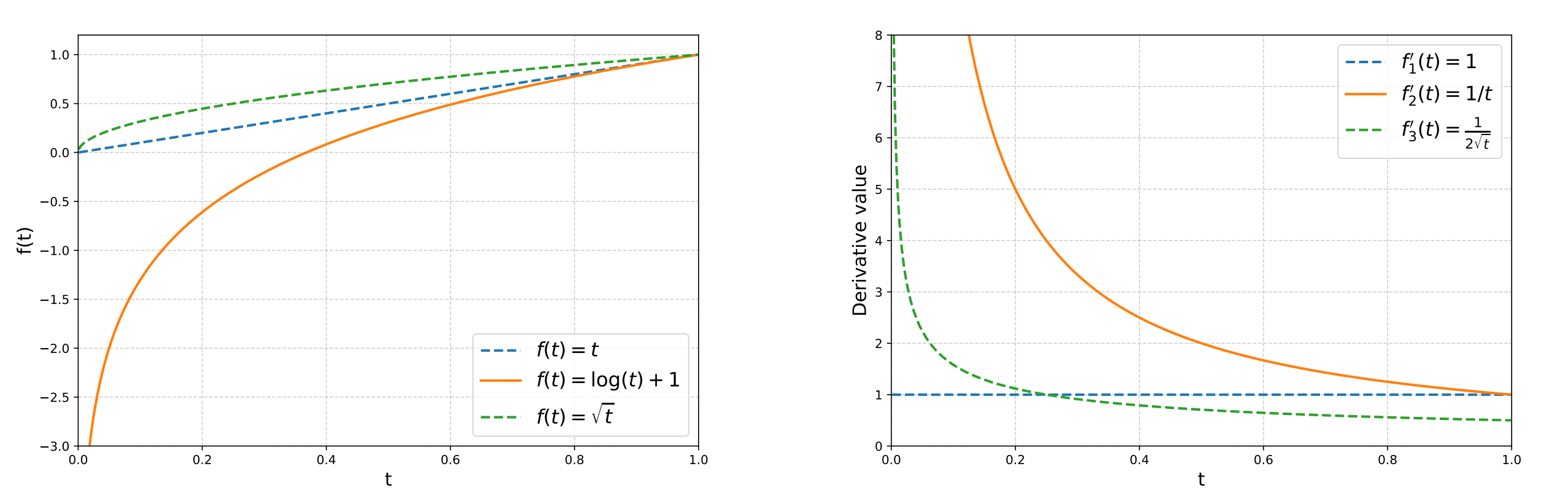
Figure 1. Choosing a non-linear objective $f(p)$ implicitly defines a prompt weight $w(p)=f’(p)$, reshaping which pass-rate regimes dominate the gradient. Example: $f(p)=\log p \Rightarrow w(p)=1/p$, emphasizing low-$p$ prompts.
Key framing. Choosing $f$ specifies which pass-rate region gets more importance through $f’(p)$.
2) Baseline and advantage: where the $(r-b)$ term comes from
We need $\nabla p_\theta(x)$. Since $p_\theta(x)=\mathbb E[r]$, the score-function identity gives \(\nabla p_\theta(x) = \mathbb E_{a\sim\pi_\theta(\cdot\mid x)}\Big[\nabla_\theta \log \pi_\theta(a\mid x)\cdot r(x,a)\Big].\)
You can subtract a baseline $b(x)$ without changing the expectation because $\mathbb E_{a\sim\pi_\theta}[\nabla_\theta \log \pi_\theta(a\mid x)]=0$. This yields the classic advantage form \(\nabla p_\theta(x) = \mathbb E_{a\sim\pi_\theta(\cdot\mid x)}\Big[\nabla_\theta \log \pi_\theta(a\mid x)\cdot (r(x,a)-b(x))\Big].\)
In practice $p_\theta(x)$ is unknown, so we use a group estimate $\hat p(x)$ and set $b(x)=\hat p(x)$.
Under the log objective, Reinforce-Ada writes the baselined gradient as \(g_{\log}(x) = \frac{1}{p_\theta(x)}\cdot \mathbb E_{a\sim\pi_\theta(\cdot\mid x)} \Big[\nabla_\theta \log \pi_\theta(a\mid x)\cdot (r(x,a)-p_\theta(x))\Big],\) which is the baseline idea with $b(x)=p_\theta(x)$, plus the outer weight $1/p_\theta(x)$ from $f’(p)$.
So the chain is already visible:
- baseline creates an advantage-like factor $(r-b)$
- $f’(p)$ multiplies the whole prompt contribution
3) Weighting: from $f’(p)$ to explicit and implicit implementations
From Section 1, the prompt weight is $w(p)=f’(p)$. Define \(\omega(x)\;:=\;w\!\big(p_\theta(x)\big)\;=\;f'\!\big(p_\theta(x)\big).\) Then \(\nabla J_f(\theta) =\mathbb E_{x\sim d}\!\left[\omega(x)\,\nabla p_\theta(x)\right] =\mathbb E_{x\sim d_\omega}\!\left[\nabla p_\theta(x)\right],\) where the implicitly reweighted prompt distribution is \(d_\omega(x)=\frac{\omega(x)\,d(x)}{\mathbb E_{x'\sim d}[\omega(x')]}.\)
This unifies implementations:
- Explicit weighting: multiply each prompt-group gradient by $\omega(x)$
- Implicit reweighting: allocate more rollouts to prompts with higher $\omega(x)$
- Hybrid strategy: use both so the effective emphasis matches $\omega(x)$
In practice the implicit path is often written as allocating group sizes $n_i$ proportional to the target weight, for example $n_i \propto 1/\hat p_i$ for the log objective. But this objective-side view still assumes that a prompt group produces a usable finite-sample update. The next issue is what happens when the sampled rewards have no variation at all.
4) Weighting alone can fail: signal collapse under small groups
4.1 Signal collapse as a gate
A practical failure mode is prompt waste: many prompt-groups produce uniform rewards (all 0 or all 1), so baseline-centered advantages are all zero. Those groups consume rollout budget but contribute no update.
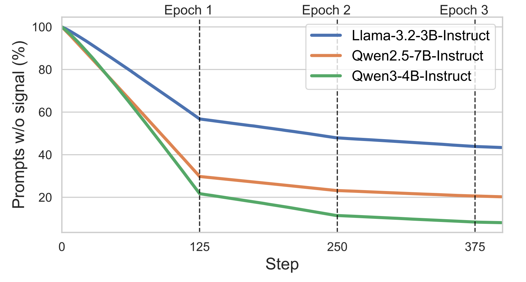
Figure 2. In sparse-reward settings, a large fraction of prompt-groups are degenerate (gate closed), so training compute is spent on samples that do not generate usable learning signal.
Suppose we estimate $p_\theta(x)$ from a group of size $G$ using \(\hat p(x)=\frac1G\sum_{i=1}^G r_i, \qquad \hat a_i = r_i-\hat p(x).\) An empirical update uses $\hat a_i$, and uses $\omega(x)\approx w(\hat p(x))$.
Define the (weighted) advantage energy as a scalar pre-gradient weight that measures usable within-group variation: \(E(x)\;:=\;w\!\big(\hat p(x)\big)\cdot \frac1G\sum_{i=1}^G \hat a_i^2 \;=\;w\!\big(\hat p(x)\big)\cdot \frac1G\sum_{i=1}^G \big(r_i-\hat p(x)\big)^2.\) For binary rewards this simplifies to \(E(x)=w\!\big(\hat p(x)\big)\,\hat p(x)\big(1-\hat p(x)\big).\) So $E(x)=0$ iff $\hat p(x)\in{0,1}$, meaning there is no within-group variation and no learning signal.
Define the gate-open event \(\mathcal O(x) =\Big\{\exists i,j: r_i\neq r_j\Big\} \quad\Leftrightarrow\quad 0<\hat p(x)<1.\) Equivalently, the gate is closed when all rewards are identical: \(\neg\mathcal O(x) \Leftrightarrow \hat p(x)\in\{0,1\}.\)
- If the gate is closed $(\neg\mathcal O(x))$: then $\hat a_i=0$ for all $i$, so the group contributes zero update under the group baseline. Any finite reweighting $\omega(x)$ is powerless because it multiplies zero.
- If the gate is open $(\mathcal O(x))$: then some $\hat a_i\neq 0$, and reweighting $\omega(x)$ can scale the resulting update.
Under Bernoulli reward with success probability $p=p_\theta(x)$, the gate opens with probability \(u(p)=\Pr(\mathcal O(x)) = 1-(1-p)^G-p^G \approx Gp\quad (p\ll 1).\) So for hard prompts (small $p$) the gate is rarely open unless you change sampling.
4.2 Gradient vs learning signal (why “non-zero update” is a separate issue)
In this note, it helps to distinguish:
- Gradient (objective-side): the true gradient of the objective you intend to optimize (e.g., $\nabla J_f(\theta)$).
- Learning signal (estimator-side): whether your finite-sample estimator produces a meaningful, non-degenerate update with acceptable signal-to-noise.
For a prompt group, a typical estimator has the form \(\hat g(x)\;\propto\;\omega(x)\cdot \frac{1}{G}\sum_{i=1}^{G}\nabla_\theta\log\pi_\theta(a_i\mid x)\,\hat a_i, \qquad \hat a_i=r_i-\hat p(x).\) When the group collapses (all $r_i$ identical), we get $\hat a_i\equiv 0$ and therefore $\hat g(x)=0$ regardless of how large the outer weight $\omega(x)$ is. This is why weighting can fail in sparse-reward regimes: it rescales gradients when they exist, but it cannot create within-group variation.
So “improving the gradient” can mean two different interventions:
- Reduce variance / noise of an unbiased estimator (allocate more samples $n_i$ where it helps; this is the variance-minimization / dynamic allocation thread).
- Increase the probability of non-degenerate samples (increase $u(p)$ via sampling rules that force mixed outcomes, or via hinting that changes $p_\theta(x,h)$).
5) Sampling: treat $n_i$ as a variance and signal discovery lever
5.1 Log-objective view: $n_i$ is for variance control
Reinforce-Ada gives a batch estimator under the log objective \(\hat g_{\text{batch}} = \frac{1}{B}\sum_{i=1}^B \frac{1}{p_i}\cdot \frac{1}{n_i} \sum_{j=1}^{n_i} \nabla_\theta \log \pi_\theta(a_{ij}\mid x_i)\,\big(r_{ij}-p_i\big), \quad p_i=p_\theta(x_i).\)
Crucially, optimization of the log objective is captured by the explicit factor $1/p_i$. The inner average is unbiased for any $n_i\ge 1$. Therefore $n_i$ does not change the target objective, it reduces estimator variance.
This is again estimator variance, not simply raw reward variance. For small $p_i$, $p_i(1-p_i)$ is small, but a finite group is likely to contain no positives and the corrected/weighted estimator can be very noisy when rare positives appear. The role of extra sampling is therefore twofold: discover non-degenerate groups and, once signal exists, reduce the variance of the weighted gradient estimate.
So adaptive sampling is a principled way to spend inference budget where it reduces noise and where it increases the chance of seeing non-degenerate groups.
5.2 Sequential sampling: stop when you find signal
Reinforce-Ada-Seq continues sampling until sufficient signal is found, for example until $K$ positive responses are collected. The paper also highlights a balanced variant that collects both positives and negatives, which is designed to avoid uniform-reward groups and preserve learning signal. Reinforce-Ada summarizes this as “by design: always collects mixed outcomes before exit”.
This is the theoretical reason sampling can beat reweighting in practice. It actively increases the frequency of non-degenerate updates rather than only amplifying their size.
However, for different prompts the number of samples $N_i$ can vary widely under adaptive sampling. This can create unstable positive to negative ratios in the retained data, which can reduce training stability and the effective batch size.
Reinforce-Ada addresses this with an Oversample, Downsample, Correct pipeline. In the gate view, the pipeline keeps both labels present in the retained group; in the variance view, it first estimates the prompt pass rate from a larger pool and then trains on a fixed-size, lower-noise subset.
-
Oversample to get a pool of $N_i$ responses and compute a high-fidelity baseline \(\tilde{p}_i = N_{\text{pos}}/N_i.\)
-
Downsample each pool to a fixed group size $n$, using balanced sampling such as $n/2$ positives and $n/2$ negatives to ensure within-group diversity. The $1{:}1$ split is best read as a robust default: the exact variance-minimizing ratio depends on the relative conditional gradient noise of the positive and negative strata, as discussed below.
Important detail. Once you select a subset (often in a label-dependent way, e.g., enforcing mixed outcomes), you have changed the effective sampling distribution of trajectories. To keep the intended objective/gradient unbiased, you must do an explicit weight correction (an importance-weight style correction) for the selection probability. For example, use the group-level acceptance rate $\tilde p_i$ to compute the selection probability and reweight accordingly.
- Correct because downsampling removes the implicit weight created by sequential sampling. Reintroduce the theoretical weight explicitly (such as multiplying by $1/\tilde p_i$ or $1/\sqrt{\tilde p_i}$).
A compact estimator view is \(\hat g(x_i) =\Big(\frac{1}{\tilde p_i}\Big)\cdot \Big(\frac{1}{n}\sum_{j=1}^{n} \nabla_\theta \log \pi_\theta(a_{j}\mid x_i)\,\big(r_{j}-\tilde p_i\big)\Big).\)
Interpretation:
- sampling finds signal and builds a robust $\tilde p_i$
- downsampling makes updates stable and balanced, but it implicitly changes the sampling distribution
- the explicit correction (weight debiasing) keeps the weighted objective consistent
5.3 Why balance positives and negatives: a variance-reduction view
The gate argument explains why a retained group needs both positive and negative rewards. There is also a more classical variance-reduction interpretation: balanced downsampling is a form of stratified sampling over the two reward strata.
Fix a prompt and write \(s(a)=\nabla_\theta \log \pi_\theta(a\mid x), \qquad \mu_+=\mathbb E[s(a)\mid r=1], \qquad \mu_-=\mathbb E[s(a)\mid r=0].\) Because $\mathbb E[s(a)]=0$, the positive and negative conditional means are tied together: \(p\mu_+ + (1-p)\mu_-=0.\) The centered prompt contribution can be written as a difference of the two conditional means: \(\mathbb E\big[s(a)(r-p)\big] =p(1-p)(\mu_+-\mu_-).\)
After oversampling, suppose the pool gives a high-fidelity pass-rate estimate, call it $p_{\mathrm{pool}}$, and the downsampled group keeps $m_+$ positives and $m_-$ negatives with $m_++m_-=n$. A natural stratified estimator is \(\hat h =p_{\mathrm{pool}}(1-p_{\mathrm{pool}})(\bar s_+ - \bar s_-),\) where $\bar s_+$ and $\bar s_-$ average score vectors over retained positives and negatives. Under the corrected pool distribution, this estimates the same centered contribution, but its variance scales roughly as \(\mathrm{Var}(\hat h\mid x) \approx p_{\mathrm{pool}}^2(1-p_{\mathrm{pool}})^2 \left(\frac{\Sigma_+}{m_+}+\frac{\Sigma_-}{m_-}\right),\) where $\Sigma_+$ and $\Sigma_-$ denote the conditional score-gradient noise in the two strata.
For fixed retained group size $n$, this means minimizing \(\frac{\Sigma_+}{m_+}+\frac{\Sigma_-}{m_-} \quad \text{s.t.}\quad m_+ + m_- = n.\) The Lagrange conditions give \(\frac{\Sigma_+}{m_+^2}=\frac{\Sigma_-}{m_-^2} \quad\Rightarrow\quad \frac{m_+}{m_-}=\sqrt{\frac{\Sigma_+}{\Sigma_-}}.\) So the variance-minimizing allocation is the usual Neyman-style rule \(m_+ \propto \sqrt{\Sigma_+}, \qquad m_- \propto \sqrt{\Sigma_-}.\) When the two conditional noises are comparable, this reduces to $m_+=m_-=n/2$, i.e., a $1{:}1$ positive/negative split. So the balanced rule is not an unconditional mathematical optimum, but a simple robust approximation to the variance-minimizing stratified allocation. It is also a way to avoid all-zero advantages and to make the positive-vs-negative contrast a low-variance estimate rather than letting one side of the contrast be represented by only a few samples.
This is the same control-variate logic as combining two unbiased estimators. If $\hat g_0$ and $\hat g_1$ are negative-side and positive-side estimates of the same prompt gradient, then an estimator \(\hat g=c_0\hat g_0+c_1\hat g_1\) is unbiased when $c_0+c_1=1$. If their variances scale like \(\mathrm{Var}(\hat g)=\left(c_0^2(1-p)^2+c_1^2p^2\right)V,\) then minimizing variance gives \(c_0=\frac{p^2}{p^2+(1-p)^2}, \qquad c_1=\frac{(1-p)^2}{p^2+(1-p)^2}.\) The estimator automatically leans on the lower-variance side, but it can only do so if both sides are present. Balanced downsampling guarantees that both conditional estimates exist with controlled finite-sample noise, while the explicit correction keeps the estimator aligned with the original pool pass rate and the target objective.
6) Two roles of adaptive sampling: weighting vs signal discovery
As discussed in Section 3, adaptive sampling can be viewed as an implicit weighting scheme: allocating more rollouts to prompts with higher target weight $\omega(x_i)=f’(p_i)$. But Section 4 revealed a deeper role. Sampling also directly increases the gate-open probability $u(p)$, which is a more fundamental way to generate learning signal than amplifying it via weighting.
6.1 Disentangling the two effects
To isolate these mechanisms, consider two variants of Reinforce-Ada:
| Variant | How it sets rollouts | Signal discovery | Weighting |
|---|---|---|---|
| Reinforce-Ada-Seq | Sequentially sample until mixed outcomes found, then downsample to fixed group size $n$ | ✓ forces mixed outcomes | ✓ corrected via explicit $1/\tilde p_i$ |
| Reinforce-Ada-Est | Estimate $\hat p_i$ from a pilot, then set $n_i\propto 1/\hat p_i$ without sequential stopping | ✗ does not guarantee mixed outcomes | ✓ same explicit $1/\hat p_i$ |
Both variants target the same weighted objective (log objective with $1/p$ emphasis). The key difference is that Reinforce-Ada-Seq forces each retained group to contain both positive and negative responses through its stopping rule and balanced downsampling, whereas Reinforce-Ada-Est merely allocates budget without ensuring the gate is open.
When comparing them, the cleanest setting is to match the total rollout budget and the final retained group size $n$.
6.2 Empirical evidence: signal matters more than weighting
| Variant | MATH500 | Minerva | Olympiadbench | AIME_misc |
|---|---|---|---|---|
| Reinforce-Ada-Seq | 0.917 | 0.530 | 0.657 | 0.388 |
| Reinforce-Ada-Est | 0.910 | 0.521 | 0.642 | 0.363 |
| GRPO (baseline) | 0.904 | 0.512 | 0.649 | 0.380 |
Table 1. Reinforce-Ada-Seq vs Reinforce-Ada-Est on Qwen3-4B. Both variants apply the same $1/\hat p_i$ reweighting, and they differ mainly in whether the sampling procedure forces mixed outcomes.
This supports the central insight: opening the gate contributes more to learning than merely scaling gradients of groups that may be degenerate.
7) Hinting: a different axis that targets the gate directly
Up to now, the “curation knobs” we discussed (weighting, adaptive sampling, sequential stopping, downsample-correct) mostly act by changing how we estimate gradients or how much compute we spend per prompt. Once you adopt the gate view, there is an equally direct but orthogonal lever: change the conditional pass rate itself so that the gate opens more often.
An easy way to remember the difference is: sampling/curation is mostly output-side (for a fixed input $x$ you change how you sample/filter $a$ or latent traces $z$), while hinting is input-side (you change the condition from $x$ to $(x,h)$).
That is why hinting fits into the same story instead of being a separate topic: sampling makes $u(p)$ larger at fixed $p$, while hinting tries to move $p$ into the regime where $u(p)$ is naturally high.
SAGE starts from standardized GRPO and makes the gate explicit.
Fix $(x,h)$. Draw $G$ rollouts with rewards $R_i\in{0,1}$. Define $\bar R$ and standard deviation $s$. Standardized GRPO uses \(A_i=\frac{R_i-\bar R}{s+\epsilon}.\)
Define the advantage energy $E=\frac{1}{G}\sum_i A_i^2$. SAGE shows \(E=\frac{s^2}{(s+\epsilon)^2},\) which collapses to 0 when $s=0$. Training behaves like a gated procedure that updates only when the group contains mixed outcomes.
Under Bernoulli rewards with success probability $p_\theta(x,h)$, \(\Pr[s>0\mid x,h]=1-(1-p_\theta(x,h))^G - p_\theta(x,h)^G,\) which is maximized at $p_\theta=1/2$, and in the sparse regime $\Pr[s>0]\approx Gp_\theta$.
7.1 What hinting changes
Sparse rewards cause GRPO to stall because many prompts have groups with no positives and advantages collapse. Privileged hinting changes the rollout distribution for such prompts while keeping the reward unchanged. A scheduler activates hints only when groups collapse. Training remains on-policy because rollouts are drawn from $\pi_\theta(\cdot\mid x,h)$. Deployment uses $h=0$ (i.e., hint strength $\ell=0$) and requires no hints.
SAGE then defines a hint distribution objective \(J_x(\theta,q)=\mathbb E_{h\sim q(\cdot\mid x)}\big[u(p_\theta(x,h))\big], \quad u(p)=1-(1-p)^G-p^G,\) and shows $u$ is strictly concave and maximized at $p=1/2$. An optimizer $q^\star_\theta$ concentrates on calibrating hints that make $p_\theta(x,h)$ as close as possible to $1/2$.
This yields a clean contrast:
- Reinforce-Ada starts from $f(p)$ and allocates compute by $f’(p)$ to optimize a non-linear transform of pass rate
- SAGE starts from standardized GRPO and optimizes the gate opening probability $u(p)$, using hints to move hard prompts out of the regime where $Gp\ll 1$
7.2 Why not sample many hints per prompt
SAGE uses Jensen’s inequality for concave $u$: \(\mathbb E_h[u(p_\theta(x,h))]\le u(\mathbb E_h[p_\theta(x,h)]).\) Intuition: for a fixed mean pass rate, mixing many hints increases variance of $p_\theta(x,h)$, and concavity of $u$ penalizes that variance, lowering expected gate openings. They therefore sample a single hint per prompt per epoch and spend compute on group size or hint strength scheduling instead.
8) Self-hinting in practice: how to generate and use hints
Self-hinting treats the hint $h$ as an additional conditioning variable that is only used during training to rescue collapsed groups. The loop has three parts: detect collapse, generate a hint, re-rollout and update.
8.1 Detect collapse (the gate)
For each prompt $x$, first roll out a group under the deployment condition $h=0$: \(a_i \sim \pi_\theta(\cdot\mid x,0),\quad r_i\in\{0,1\},\quad \hat p(x)=\frac{1}{G}\sum_{i=1}^G r_i.\) Define collapse by the gate condition: \(\text{collapse}(x)\; \Leftrightarrow\; \hat p(x)\in\{0,1\}\; \Leftrightarrow\; s=0.\) Only when collapse happens do we activate hinting.
8.2 Generate a hint from the model itself
When collapse is detected on prompt $x$, we generate a training-only hint $h$ from a hint policy $q_\phi(h\mid x)$. In self-hinting, $q_\phi$ is implemented by the model itself in a dedicated “hint mode” that is allowed to condition on the optimal solution $y^\star$ (privileged information): \(h \sim q_\phi(\cdot\mid x, y^\star)\approx \pi_\theta(\cdot\mid \texttt{HintPrompt}(x,\ell, y^\star)).\)
Here $y^\star$ is the reference (optimal) solution used only to produce a hint. A practical template family is to control hint strength by a level $\ell\in{1,2,3}$.
Crucially, the hint is not rewarded and does not change the task reward definition. The reward remains the same function of $(x,a)$ as in the no-hint setting: \(r=r(x,a),\quad a\sim \pi_\theta(\cdot\mid x,h).\)
8.3 Re-rollout under the hint and update on-policy in $(x,h)$
Given the generated hint, roll out a new group: \(a_i \sim \pi_\theta(\cdot\mid x,h),\quad r_i=r(x,a_i).\) Then apply the same update rule as usual, but now on the hinted condition: \(\Delta \theta \propto \sum_{i=1}^{G}\nabla_\theta\log \pi_\theta(a_i\mid x,h)\cdot A_i(x,h).\) This is on-policy in the augmented space $(x,h)$ because samples are drawn from $\pi_\theta(\cdot\mid x,h)$.
8.4 Keep deployment clean: always evaluate and deploy with $h=0$
Training uses hinting only as a rescue path. Deployment and most evaluation use: \(h=0,\quad a\sim \pi_\theta(\cdot\mid x,0).\) The key question becomes generalization from hinted rollouts back to the no-hint condition. Two standard practices help:
- Hint dropout or annealing: gradually reduce the probability of triggering hinting over training, so the model increasingly succeeds under $h=0$.
- Hint-only-on-collapse: never use hints when the gate is already open, preventing over-reliance on hints where learning signal already exists.
Two plots at the end: RL efficiency curves
The two figures below are often described as improving compute efficiency: you spend fewer rollouts on degenerate groups (closed gate) and more rollouts on conditions that actually produce learning signal. But the deeper point is that they improve the RL efficiency curve itself: for a fixed training compute budget you get higher performance, or equivalently you reach the same performance with fewer rollouts. This is improving the scaling law of performance vs compute, not just moving along the same curve.
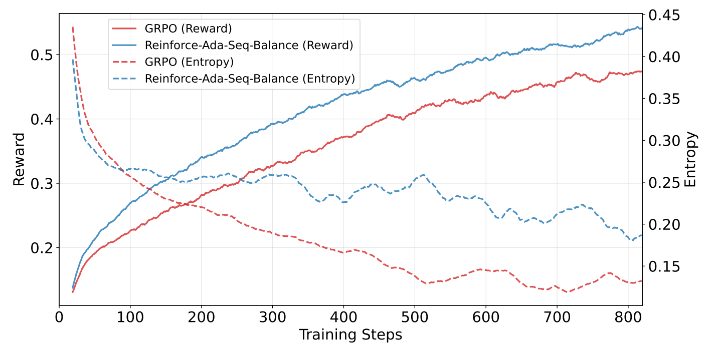
Figure 3. Reinforce-Ada-style adaptive sampling/downsample-correct reduces wasted rollouts and stabilizes updates. Interpreting it as “compute efficiency” is correct, but the net effect is an upward shift in the performance-vs-compute curve.
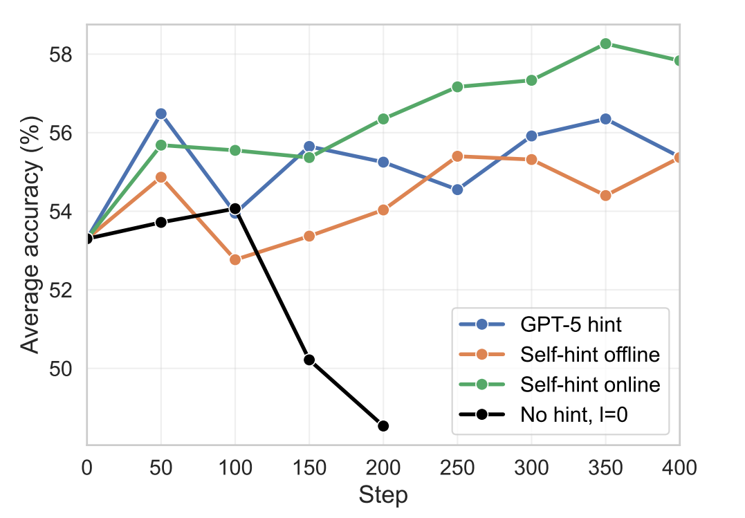
Figure 4. Self-hinting targets the gate directly by changing the condition $x\to (x,h)$ only when collapse is detected. This looks like compute efficiency (more open-gate groups per rollout) and acts like an improvement of the RL efficiency curve (more learning per unit compute).
A unified view of curation knobs
The whole story can be read as the interaction between opening the gate and reducing variance. Gate-opening decides whether a finite group produces any usable update at all; variance reduction decides how noisy that update is once it exists. Sampling, downsampling, weighting, and hinting differ mainly in which side they touch first.
You can summarize the full chain as five knobs that appear naturally from the math:
- Choose $f$ to define what you value across prompt difficulty via $f’(p)$
- Choose a baseline to form an advantage-like term $(r-b)$, reducing variance and stabilizing learning
- Use adaptive sampling to spend inference budget where it increases signal discovery and reduces estimator variance, including sequential rules that force mixed outcomes
- Use downsampling with correction to keep static training throughput while preserving the weighted objective
- Use hinting when standardized GRPO behaves like a gate and hard prompts have $Gp\ll 1$. Hints aim to calibrate $p$ toward $1/2$ and open the gate more often
Miscellaneous notes
GRPO
In the Bernoulli pass-rate view, standardized advantages induce an effective emphasis roughly proportional to $1/\sqrt{p(1-p)}$, which corresponds to $f(p)=2\arcsin(\sqrt{p})$ up to normalization and estimator details.
When does the gate become the bottleneck?
For Bernoulli rewards with pass rate $p$ and group size $G$,
\(u(p)=1-(1-p)^G-p^G \approx Gp \quad (p\ll 1).\)
A useful rule of thumb is that the gate is meaningfully open only when $Gp$ is not too small.
For example, $Gp\approx 1$ gives $u(p)\approx 1-e^{-1}\approx 0.63$ (ignoring the $p^G$ term), while $Gp\ll 1$ means most groups are degenerate and any weighting becomes ineffective.
Why downsample at all?
Sequential or oversized pools stabilize $\hat p$ but create highly variable per-prompt compute and skewed class ratios (mostly negatives on hard prompts, mostly positives on easy prompts).
Downsampling to a fixed group size $n$ restores stable training throughput and balanced within-group variation, while the explicit correction factor (e.g., $1/\tilde p$ for log objective) preserves the intended objective emphasis.
Group size $G$: signal vs throughput
Increasing $G$ raises $u(p)$ and reduces variance of $\hat p$, but it also reduces the number of distinct prompts per batch under a fixed rollout budget.
This creates a trade-off: larger $G$ improves within-prompt signal discovery, while smaller $G$ improves prompt coverage. Adaptive sampling and downsample-correct can decouple these two axes.
Hinting vs sampling: two orthogonal levers on $u(p)$
Both aim to increase gate openings $u(p)$, but through different control knobs:
- Sampling increases effective $G$ or enforces mixed outcomes (changing the estimation process).
- Hinting changes $p_\theta(x,h)$ by altering the input/condition while keeping the reward definition unchanged.
A simple mental model is: sampling makes $u(p)$ larger at fixed $p$, while hinting moves $p$ toward the regime where $u(p)$ is maximized (near $1/2$).
On-policy note
If hints are treated as additional conditioning $h$ and rollouts are sampled from $\pi_\theta(\cdot\mid x,h)$, the update remains on-policy in the augmented space $(x,h)$.
The deployment distribution corresponds to $h=\ell=0$, so the key question shifts to generalization across $h$, not off-policy correction.
Choosing $f$
The derivative $w(p)=f’(p)$ is the real knob.
- Log: $w(p)=1/p$, strongly emphasizes low-$p$ prompts.
- Power: $f(p)=p^\alpha\Rightarrow w(p)=\alpha p^{\alpha-1}$ (tunable emphasis).
- Symmetric around $1/2$: designs that emphasize uncertain prompts can be aligned with the gate view.
In practice, overly singular $w(p)$ may amplify noise when $\hat p$ is estimated from small groups, motivating oversample + smoothing or clipping.
Since this is out of the scope of the original papers, we have not deeply explored the design space of $f$ and $w$. It would be interesting to see how different choices interact with sampling and hinting.
Practical detail: smoothing / clipping $\hat p$
When $w(p)$ is steep near 0 or 1 (e.g., $1/p$), small-sample $\hat p$ can cause unstable weights.
Common fixes include $\hat p\leftarrow \mathrm{clip}(\hat p,\delta,1-\delta)$ or Bayesian smoothing $\hat p=(k+\alpha)/(G+\alpha+\beta)$.
These do not change the conceptual story, they stabilize finite-sample implementations.
Unifying “advantage energy” across baselines
With group baseline $b=\hat p$, Bernoulli rewards yield \(\frac{1}{G}\sum_i (r_i-\hat p)^2 = \hat p(1-\hat p).\) With standardized GRPO $A_i=(R_i-\bar R)/(s+\epsilon)$, \(E=\frac{1}{G}\sum_i A_i^2=\frac{s^2}{(s+\epsilon)^2}.\) Both collapse to 0 exactly when within-group variability vanishes ($s=0$ or $\hat p\in{0,1}$), making the “gate” interpretation consistent across estimators.
Acknowledgement: thanks to the collaborators of the works for helpful discussions and feedback on this note.
References
[1] Optimizing Chain-of-Thought Reasoners via Gradient Variance Minimization in Rejection Sampling and RL. [Link]
[2] Reinforce-Ada: An Adaptive Sampling Framework under Non-linear RL Objectives. [Link]
[3] Self-Hinting Language Models Enhance Reinforcement Learning. [Link]
Citation
If you build on the ideas here, please cite the original papers ([1]–[3]). If this note is useful as a pointer/synthesis, you can also cite the blog post.
BibTeX
@misc{dong2026curatelearningsignal,
   title = {Curate the Learning Signal for Reinforcement Learning},
   author = {Dong, Hanze},
   year = {2026},
   month = {February},
   url = {https://hendrydong.github.io/blogs/pages/rl-ada.html},
   note = {Blog post on Hanze Dong's Blogs},
   urldate = {2026-02-25}
}